Machine Learning for Customer Engagement: OML Classification Tutorial

By: Jacob Beasley, Director at Centroid and Kyle Berndt, Principal Consultant at Centroid — August 11, 2026

Using Machine Learning to Predict Affinity Card Adoption 

Machine learning (ML) is a powerful tool that can have a variety of methods and uses. In this article, we share strategies for using machine learning for “classification”. In the context of machine learning, classification creates a model that can perform as a sorting machine, utilizing features of the data to categorize them. 

We will walk you through using machine learning to predict customers of a fictional company who are likely to be interested in signing up for an affinity card program. The machine learning model will be given access to a set of data about existing customers, including information about their household size, occupation, and which products they have previously purchased. The model will train on that data and learn to recognize patterns about which other data points correlate with the likelihood that customers sign up for the affinity card or not. 

Using Oracle Machine Learning UI for training and using models 

The Oracle Machine Learning (OML) UI is a powerful interface designed to allow users to turn their Oracle database into a powerful tool for predictive analytics using machine learning,. It includes tools to make developing machine learning models easy.  

One of those features is their notebooks, which are powerful workspaces allowing users to collaborate and work on tasks in a managed environment with built-in tools to make it easy to connect to the database and run ML tasks in Python, R, and SQL.

One of the most cumbersome parts about making use of machine learning models is tuning the models by figuring out the optimal parameters for training it. That is where Oracle’s AutoML experiments come into play. AutoML Experiments are a feature of the OML UI that allow you to configure a set of fundamental settings regarding how you want your model trained, such as what data you are trying to predict, and what data points should be ignored. Then, it will take those settings and automatically train and test several iterations of models for the use case, allowing the user to pick and choose from the most effective models, without the need for the manual training and testing of an extensive number of iterations of the model. 

Hands-On Tutorial 

In this section, we’ll walk you through how to run a simple machine learning experiment in the OML UI. We’ll leverage the SH. SUPPLEMENTARY_DEMOGRAPHICS table to predict the likelihood of a customer signing up for an affinity card (loyalty card). 

The SH schema, including the SUPPLEMENTARY_DEMOGRAPHICS table, are built into Oracle’s Autonomous AI databases, so you can follow along in your own database’s OML UI. 

Setup 

You will need a database user with access to the OML UI. In the Oracle Cloud UI, you can find your database, and in the upper right-hand corner, go to Database Actions > Database users. Once there, create or edit the user you want to use, and make sure they have the ‘OML’ access toggled on   

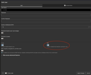
After your user is set up, you will need to find your OML UI ‘s URL. Return to your database details in the Oracle Cloud Console, and navigate to the Tool configuration tab. Once there, find the Public Access URL under Oracle Machine Learning user interface. Navigate to that URL in your web browser, and use the username and password for the user to set up in the previous step to sign in. Under Quick Actions on the home page, select Notebooks to navigate to your user’s list of notebooks. Once there, use the Create button to make a new notebook, name it “Affinity Card Demo”, or another name of your choice, and after creating it, you are ready to get into the demo.              

Setting Up and Examining the Data 

1. In the first paragraph of this notebook, we’ll import the necessary python libraries. When using a notebook session, many of the python libraries relevant to machine learning are already available without needing to install them. 

%python  

# Import the relevant Python packages (these are all pre-installed when using a notebook session in the OML UI.)  

import pandas as pd  

import oml  

import warnings  

# Filter out warnings about future changes in behavior to reduce clutter in output  

warnings.simplefilter(action=’ignore’, category=FutureWarning) 

2. Next, we’ll call oml.sync() to load the data from the table into a dataframe and show the loaded data. 

You can take an opportunity to look through the data here. This table contains demographic information such as the education level and household size for the customers. It also contains information about which products the customer has previously purchased.

%python 

DEMO = oml.sync(table = ”SUPPLEMENTARY_DEMOGRAPHICS”, schema = ”SH”) 

z.show(DEMO.head()) 

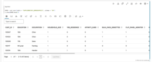
3. In the next paragraph, we’ll calculate some statistics about the data, such as the mean (average) and standard deviation. In this case, since a lot of the columns are Boolean values, the mean also doubles as telling you what percentage of users have that column as true. 

%python 

summary_df = DEMO.describe() 

summary_df = summary_df.reset_index() 

summary_df = summary_df.rename(columns = {‘index’: ’Statistic’}) 

z.show(summary_df.head()) 

4. OML UI gives you the ability to visualize data in several different ways, including several types of graphs. To do this, select the icons for the graph type you would like, and customize the exact settings you would like. For this notebook paragraph, let’s look at a bar graph of how many customers have signed up for the affinity card.  

Graph settings:
-  Series to Show: count
- Group by: AFFINITY_CARD 

%python 

z.show(DEMO.crosstab(‘AFFINITY_CARD’)) 

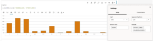
5. We can use these graphs to visualize more interesting things as well. In this case, we’ll use it to looks for patterns in how household size correlates to customers with affinity card holders. 

Each column represents users who meet both the affinity card status and household size on the axis. For example, the first column is users who do not have an affinity card and have a household size of one. 

If you want to examine the data further, switch out HOUSEHOLD_SIZE with some of the other columns and explore patterns regarding which data points correlate to whether or not customers have affinity cards. 

Graph settings: 

Aggregate Duplication: Last 

Series to Show: count 

Group By: AFFINITY_CARD, HOUSEHOLD_SIZE (order matters) 

%python 

z.show(DEMO.crosstab([‘HOUSEHOLD_SIZE’, ’AFFINITY_CARD’

Training the Model 

Now that we have loaded in the information from the database and looked at it, let’s put it to use in training a model. 

1. First, we’ll create a new dataframe containing only the information relevant to our machine learning model. In this case, we are simply excluding the comments column. 

%python 

# Creates a new dataframe with only the specified columns 

DEMO_DF = DEMO[[ 

    ”CUST_ID”, 

    ’AFFINITY_CARD’, 

    ”BOOKKEEPING_APPLICATION”, 

    ”BULK_PACK_DISKETTES”, 

    ”EDUCATION”, 

    ”FLAT_PANEL_MONITOR”, 

    ”HOME_THEATER_PACKAGE”, 

    ”HOUSEHOLD_SIZE”, 

    ”OCCUPATION”, 

    ”OS_DOC_SET_KANJI”, 

    ”PRINTER_SUPPLIES”, 

    ”YRS_RESIDENCE”, 

    ”Y_BOX_GAMES” 

    ]] 

2. Next, we’ll separate our data into training and testing data. What we are accomplishing here is splitting our data into two pools, one of which we will use to train the model, and the second we will use to validate it. 

%python 

# This splits the dataframe into 2 pools, TRAIN with 60% of the data, and TEST with the other 40%  

TRAIN, TEST = DEMO_DF.split(ratio = (0.6,0.4)) 

# Our training data will exclude the AFFINITY_CARD column 

TRAIN_X = TRAIN.drop(‘AFFINITY_CARD’) 

# The column we will try to predict based on the other columns is AFFINITY_CARD 

TRAIN_Y = TRAIN[‘AFFINITY_CARD’] 

# The TEST data will be unmodified, with the AFFINITY_CARD column being set as its “answer” 

TEST_X = TEST 

TEST_Y = TEST[‘AFFINITY_CARD’] 

3. Now that the data is prepared, we’ll use it to train a model. This paragraph will train a model using the decision tree algorithm with default settings using the training data prepared in the previous step. 

The displayed output displays details about the model and its settings. For this demo, we are going to go with the default settings for the sake of simplicity. Iterating on tuning these settings would allow you to improve your model’s accuracy. 

%python 

# Clean up model from previous runs if it exists 

try: 

    oml.drop(model = ’AFFINITY_DT_MODEL’) 

except: 

    print(“No pre-existing model found”) 

# Create dt (Decision Tree model) with default settings 

setting = dict() 

dt_mod = oml.dt(**setting) 

dt_mod.fit(TRAIN_X, TRAIN_Y, case_id = ’CUST_ID’, model_name = ’AFFINITY_DT_MODEL’)

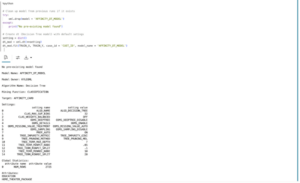
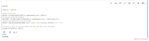
4. Now that we have a model trained, let’s see how well it did. This paragraph makes predictions on the TEST dataset that we created earlier and then displays the overall score. In this case, it was able to accurately predict whether a customer had an affinity card for more than 82% of the test cases. 

%python 

case_id = ’CUST_ID’ 

# Make Predictions 

RES_DF = dt_mod.predict(TEST_X, supplemental_cols = TEST_X) 

# Find the predicted probability 

RES_PROB = dt_mod.predict_proba(TEST_X, supplemental_cols = TEST_X[case_id])  

# join the predictions and probability predictions 

RES_DF = RES_DF.merge(RES_PROB, how = ”inner”, on = case_id, suffixes = [“”, ””]) 

# Display a score for how accurately the data was able to be predicted 

dt_mod.score(TEST_X, TEST_Y) 

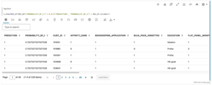
5. Let’s take a closer look at how the test data was used in the next paragraph. The RES_DF that we created shows the predictions made on the test data. It contains a copy of the data in the testing data set, along with the added columns of PREDICTION, PROBABILITY_OF_1, and PROBABILITY_OF_0. The PREDICTION column indicates whether the model predicted the customer to have an affinity card or not, and the two PROBABILITY_OF_X columns indicate how likely the model thought that X was the correct value for that customer. 

%python 

# Show predictions on the test dataset. 

# Filtering to include only results where the predicted likelihood of having an affinity card if over 50% 

# Pull the PREDICTION and PROBABILITY OF_1 columns to the front for convenience. 

z.show(RES_DF[RES_DF[‘PROBABILITY_OF_1’] > 0.5][[‘PREDICTION’, ’PROBABILITY_OF_1′] + RES_DF.columns]) 

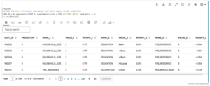
6. Next, we’ll take a closer look at some of the factors which influenced the model’s predictions. The table we are generating with this script will show the predictions the model made for customers, along with the 3 data points that had the largest impact on reaching that prediction.

This table has NAME_X and VALUE_X columns that indicate which data point was considered and what that customer’s value for it was. The WEIGHT_X column indicates how strongly that data point was considered in the prediction. The higher the positive weight is, the more powerful that data point was considered in reaching the prediction. Conversely, the lower negative weights indicate that the data point was considered to reduce the likelihood of the given prediction. 

Take a moment to review the crosstab we created in step 5 of the previous section. You’ll notice that many of these weights are intuitive based on patterns you may have noticed. For example, amongst customers with a HOUSEHOLD_SIZE of 2, around 1000 did not have an affinity card and around 100 did. With such a drastic difference in adoption rate at that HOUSEHOLD_SIZE, it makes sense that is weighted so heavily as evidence towards the first 4 customers depicted below being predicted to not be affinity card holders. 

%python 

# Show the top 3 attributes considered, and their impact on the prediction 

RES_DF = dt_mod.predict(TEST_X, supplemental_cols = TEST_X[[‘CUST_ID’]], topN_attrs = 3) 

z.show(RES_DF) 

Making Use of the Model’s Predictions 

Our fictional company wants to promote their affinity cards by sending out fliers to customers who are not already members of the affinity program. For our sample data set, that would be 3,428 customers out of our total 4,500. As a cost-saving measure, the company only wants to send the fliers to customers who are likely to act on them. 

We can use the model trained above to predict the likelihood each of the customers without an affinity card would sign up for one. Then, our company can use these predictions to only send fliers out to the customers who meet a threshold for likelihood of signing up. 

1. We’ll start by creating a new OML DataFrame. This time, instead of syncing the entire table, we’ll only include the customers who do not currently have an affinity card.

%python 

CARDLESS_CUSTOMERS = oml.sync(query=”SELECT * from SH.SUPPLEMENTARY_DEMOGRAPHICS where AFFINITY_CARD = 0″) 

z.show(CARDLESS_CUSTOMERS.head()) 

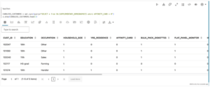
2. Now that we have our customers, we’re going to run predictions against. This will look very similar to what we did when we were testing the model after training it earlier. We are going to look for customers who were predicted to have a 35% or higher in their PROBABILITY_OF_1. This cuts our list down from 3.428 to 791 customers. This reduces the total number of fliers we will send out by around 75%, and we will expect a high follow-up rate on those fliers. 

%python 

case_id = ’CUST_ID’ 

# Make Predictions 

CARDLESS_CUSTOMERS_RES_DF = dt_mod.predict(CARDLESS_CUSTOMERS, supplemental_cols = CARDLESS_CUSTOMERS) 

# Find the predicted probability 

CARDLESS_CUSTOMERS_RES_PROB = dt_mod.predict_proba(CARDLESS_CUSTOMERS, supplemental_cols = CARDLESS_CUSTOMERS[case_id]) 

# join the predictions and probability predictions 

CARDLESS_CUSTOMERS_RES_DF = CARDLESS_CUSTOMERS_RES_DF.merge(CARDLESS_CUSTOMERS_RES_PROB, how = ”inner”, on = case_id, suffixes = [“”, ””]) 

# Filtering to include only results where the predicted likelihood of getting an affinity card is at least 35% 

# Pull the PREDICTION and PROBABILITY OF_1 columns to the front for convenience. 

z.show(CARDLESS_CUSTOMERS_RES_DF[CARDLESS_CUSTOMERS_RES_DF[‘PROBABILITY_OF_1’] >= 0.35][[‘PREDICTION’, ’PROBABILITY_OF_1′] + CARDLESS_CUSTOMERS_RES_DF.columns] 

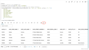
3. At this point, we now know the customers we want the fliers to be sent to but still need to get this information to our marketing team. We will join the list of users we made predictions on to the SH.CUSTOMERS table, which contains the information about these fictional customers to get their addresses.  

For the sake of keeping our demo simple, we will simply download the table of results, which we could then forward to the marketing team. For a real-world application, we would likely automate this report to run on a schedule, and upload the information to the system that the marketing team uses. 

%python 

# Create a reference to the CUSTOMERS table 

CUSTOMER_INFO = oml.sync(schema=”SH”, table =”CUSTOMERS”) 

# Find the customers we intend to send fliers to, and return their address information 

FLIER_CUSTOMERS_REPORT = FLIER_CUSTOMERS.merge(CUSTOMER_INFO, how = ”left”, on = ’CUST_ID’, suffixes = [“”, ””])[[ 

    ”CUST_ID”, 

    ”CUST_FIRST_NAME”, 

    ”CUST_LAST_NAME”, 

    ”CUST_STREET_ADDRESS”, 

    ”CUST_POSTAL_CODE”, 

    ”CUST_CITY”, 

    ”CUST_CITY_ID”, 

    ”CUST_STATE_PROVINCE” 

    ]] 

z.show(FLIER_CUSTOMERS_REPORT)  

AutoML Experiments Tutorial

When we trained the model earlier, we ran with a decision tree model with the default setting. To ensure the model we created is as accurate as possible, it is a good idea to try multiple machine learning algorithms and settings. Keep in mind, if we had to go through the process we ran through in the tutorial above, it would be very time-consuming and tedious.

That is where Oracle’s AutoML Experiments come in. This tool allows you to configure settings for making predictions and will run through multiple attempts to train models for it using a variety of algorithms and settings.

Let’s see how much faster and easier it is to train models for our affinity card use case using AutoML Experiments instead of manually.

Create and Run the Experiment

1. In the OML UI, use the navigation menu in the top left and go to Project > AutoML Experiments. Use the ‘Create’ button to create a new experiment. Use these settings to replicate our predictions from the first demo, and then Save using the button in the upper right.

a. Name: Affinity Card AutoML Demo (or your choice)

b. Data Source: SH for the schema, SUPPLEMENTARY_DEMOGRAPHICS as the table

c. Predict: AFFINITY_CARD

d. Prediction Type: Classification

e. Case ID: CUST_ID

f. Additional Settings:

i. Database Service Level: Medium

ii. Model Metric: Balanced Accuracy*

iii. Leave the rest as defaults

g. Features

i. uncheck COMMENTS

*Balanced accuracy is not directly comparable to the score we were using for our initial manual experiments, but provides us with a more insightful metric, as it adjusts for imbalances in the data, such as relatively large number of users without affinity cards relative to the number of users with affinity cards in this dataset.

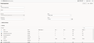
2. In the upper right corner, use the start button to start running the experiment. For this demo, use the Faster Results option to reduce the length of time you’ll need to wait for the experiment to complete. Wait for the experiment to complete before moving to the next step. This will take several minutes.

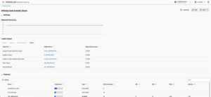
3. Once complete, a new screen with the results will appear. The main two things to focus on here are the Leader Board and the Features list

Under the Leader Board, you can see the top models that the AutoML experiment tried in its run and how well they did.

Under the Features section, you can see metrics on the data points used for training the model. One of the most interesting things here is the Importance column, as that indicates how impactful the data point is when making predictions. In this AutoML experiment, the household size was found to be the most important datapoint for predicting customers who would be likely to sign up for an affinity card.

Deploying a model from an AutoML to make predictions by API

After the great success we had in optimizing who the marketing fliers sould be mailed to, our fictional company is trying to further increase the reach of their affinity card program. They want the ability to predict if a customer is likely to sign up for an affinity card in real time.

This allows us to retrieve predictions about customers in real time. Let’s put one of our models from our AutoML experiment to use to meet this need.

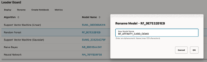
1. We had 2 models tied for the highest balanced accuracy. We’ll leverage the model using the random forest algorithm for this tutorial.

We’ll start by giving the model a new name other than the one that was generated by the AutoML Experiment. Select the row in the Leader Board for the model, and then use “Rename” button to change the name to a more specific one like RF_AFFINITY_CARD_DEM

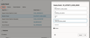
2. Next, we’ll deploy this model to our database’s restful services. Select the row for the model in the Leaderboard once more, and this time use the “Deploy” button.

a. Name: RF_AFFINITY_CARD_DEMO

b. rf_affinity_card_demo

c. version: 1.0

d. Namespace: Your database schema’s name

e. Shared: checked

Using the deployed model using Oracle DB’s Restful services

For the sake of having a simple demo, we will use curl to access the model we deployed in the previous step to make predictions. In a production use case, this same integration would be done as an integration with your application rather than through this manual process.

To avoid differences in environments, it is recommended to follow along using a cloud shell in your Oracle Cloud tenancy.

1. First, we need to retrieve your database’s RESTful services URL. This can be done by taking the URL for your OML UI, and removing everything after the “.com”.

2. In your cloud shell, create a file called oml.env using the template below. We’ll use it to keep the configuration for connecting to our database’s RESTful services. Fill it in with the values appropriate for your environment. Once complete, run `source oml.env` to load it into your session.

a. oml_username: the username you used to sign into the OML UI

b. oml_password: the password you used to sign into the OML UI

c. omlservice: the URL retrieved in the previous step

3. Next, we’ll request an access token for our user using this curl command. Note, this token will expire after 1 hour.

Validate that the step above worked by calling `echo $token`. You should see a long string of characters.

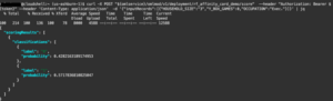
Now we can call our model through its scoring restful endpoint. This endpoint will accept the parameters it is trained on and make a prediction on it. In this case, it predicted a roughly 57% chance of the customer being interested in an affinity card.

Turn Insight into Impact

You’ve seen how machine learning can uncover patterns, improve targeting, and drive smarter decisions; now it’s your turn to apply it. Whether you’re optimizing marketing efforts, enhancing customer experiences, or exploring new predictive use cases, the tools are in your hands.

Start building, start experimenting, and start delivering results. Reach out to Centroid to unlock the power of machine learning in your Oracle environment and build unique, high-impact use cases tailored to your specific business needs. Your next breakthrough could be just one model away.